Clay (Matlock, 1970)
The p-y curve for clays according to Matlock for static loading is shown in Figure 1.
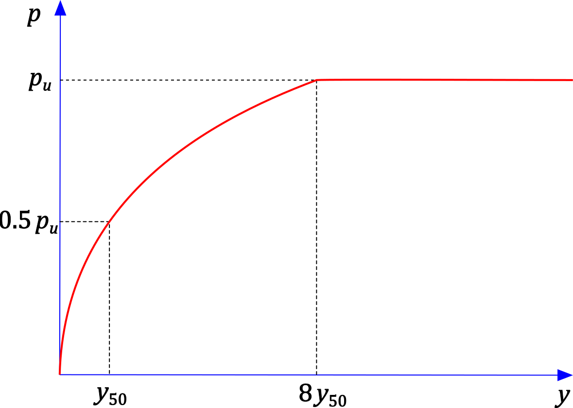 Figure 1: p-y curve for clay (Matlock, 1970)
The input parameters for determining the curve are:
d [m] | – | pile diameter |
z [m] | – | depth below the ground surface |
γ [kN/m3] | – | unit weight of the soil |
cu [kPa] | – | undrained shear strength of the soil |
ε50 | – | strain corresponding to one-half of the ultimate soil resistance pu |
J | – | empirical factor (typically 0.5) |
The reference displacement y50 is given by:

The ultimate soil resistance pu is taken as the smaller of the values:

The parabolic part of the curve is described by:
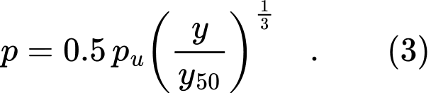
The curve given by equation (3) reaches the ultimate soil resistance pu at a displacement of y = 8y50. Beyond that point, the curve has a constant value of pu.
This p-y curve also has a variant for cyclic loading, whose shape is shown in Figure 2.
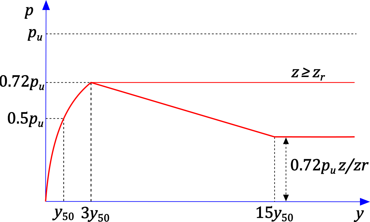 Figure 2: p-y curve for clay (Matlock, 1970) for cyclic loading
For this variant, the ultimate soil resistance is reduced to 0.72pu.
The curve given by equation (3) reaches p = 0.72pu at a displacement of approximately y = 3y50.
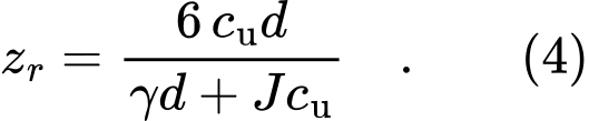
In addition, a transition depth zr is defined, which marks the boundary between two types of curve shape. At depths less than zr, after reaching p = 0.72pu, the curve decreases linearly and reaches a value of 0.72pu·z/zr at y = 15y50. At depths greater than zr, the curve remains constant at p = 0.72pu once this value has been reached. This shape is shown in Figure 2.
The transition depth zr is given by: