


Jointed Rock (JR)
The Jointed Rock constitutive model belongs to the class of constitutive models used to describe the mechanical behavior of jointed rock masses. It combines the elastic–perfectly plastic Mohr–Coulomb model, which represents the isotropic rock matrix, with the interface Mohr–Coulomb model, which describes the mechanical response of a predefined joint. The model assumes locally isotropic elastic behavior governed by the stiffness of the intact rock, while plastic anisotropy can be introduced by assigning different strength properties to different directions. Up to two joints with distinct orientations can be specified. The required material parameters are listed in the following table.
Symbol | Units | Description | |
Intact rock | |||
E | [MPa] | Modulus of elasticity | |
Eur | [MPa] | Modulus of elasticity in unloading/reloading | |
ν | [-] | Poisson’s ratio | |
c | [kPa] | Effective cohesion | |
φ | [°] | Effective angle of internal friction | |
ψ | [°] | Angle of dilation | |
σt | [kPa] | Maximum allowable tensile strength | |
TsRF | [-] | Tensile strength reduction factor | |
αt | [1/°C] | ||
Joint (failure surface) | |||
c | [kPa] | Effective cohesion | |
φ | [°] | Effective angle of internal friction | |
ψ | [°] | Angle of dilation | |
σt | [kPa] | Maximum allowable tensile strength | |
TsRF | [-] | Tensile strength reduction factor | |
β | [°] | Joint dip | |
For the two-dimensional plane-strain state considered here, the orientation of a single joint in the Cartesian coordinate system is defined by the dip angle β, measured counterclockwise from the horizontal x-axis, as illustrated in the following figure. The strike angle does not need to be specified explicitly, as it is fixed at 90° under the adopted plane-strain assumption.
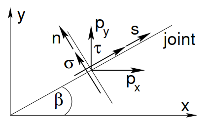 Single joint (failure surface) in the cartesian coordinate system showing surfaces tractions px, py and joint stresses τ, σ in the s, n coordinate system
The shear τ and normal σ stresses in the local joint coordinate system are then written in terms of the cartesian stresses as follows


Using the local joint stresses, namely the shear stress τ and the normal stress σ, the joint failure criterion can be formulated in terms of the shear strength parameters–cohesion cj and friction angle φj–together with the tensile strength σt,j, which defines the tension cut-off. The resulting shear and tensile failure surfaces are illustrated in the following figure.
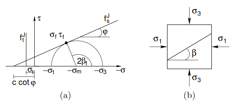 a) Shear fsJ and tensile ftJ failure surfaces, b) Rock segment loaded in biaxial compression
As described in the Theoretical manual the standard Mohr-Coulomb failure criterion of the intact matrix is formulated in terms of the principal stresses. The following equation provides relationship between cartesian σ principal σI stresses in the form
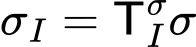
where TIσ is the corresponding transformation matrix, see the Theoretical manual for further details.
Expressing both the joint and matrix failure criteria in terms of the Cartesian stress components facilitates their simultaneous treatment within a multisurface plasticity framework. Each joint introduces three possible combinations of active yield surfaces: shear failure, tensile failure, and simultaneous shear and tensile failure. In addition, the Mohr–Coulomb model with a tension cut-off gives rise to nine possible combinations of active failure surfaces. Consequently, the combined formulation requires up to 159 distinct combinations to be examined sequentially.
When the joint and matrix failure criteria are simultaneously active, the principal directions of the trial stress state and the updated stress state generally no longer coincide. Consequently, local iterations are required at each material point to determine the updated stress state, even though both constitutive components belong to the class of elastic–perfectly plastic models.
Details on numerical implementation can be found in the Theoretical manual.